Warning: include(): open_basedir restriction in effect. File(/home/matlabsite/public_html/wp-content/plugins/wp-super-cache/wp-cache-base.php) is not within the allowed path(s): (/home/h321874/:/tmp:/var/tmp:/opt/alt/php81/usr/share/pear/:/dev/urandom:/usr/local/lib/php/:/usr/local/php81/lib/php/) in /home/h321874/domains/matlabsite.com/public_html/wp-content/plugins/wp-super-cache/wp-cache.php on line 95

Warning: include(/home/matlabsite/public_html/wp-content/plugins/wp-super-cache/wp-cache-base.php): failed to open stream: Operation not permitted in /home/h321874/domains/matlabsite.com/public_html/wp-content/plugins/wp-super-cache/wp-cache.php on line 95

Warning: include(): Failed opening '/home/matlabsite/public_html/wp-content/plugins/wp-super-cache/wp-cache-base.php' for inclusion (include_path='.:/opt/alt/php72/usr/share/pear') in /home/h321874/domains/matlabsite.com/public_html/wp-content/plugins/wp-super-cache/wp-cache.php on line 95

Warning: include_once(): open_basedir restriction in effect. File(/home/matlabsite/public_html/wp-content/plugins/wp-super-cache/ossdl-cdn.php) is not within the allowed path(s): (/home/h321874/:/tmp:/var/tmp:/opt/alt/php81/usr/share/pear/:/dev/urandom:/usr/local/lib/php/:/usr/local/php81/lib/php/) in /home/h321874/domains/matlabsite.com/public_html/wp-content/plugins/wp-super-cache/wp-cache.php on line 122

Warning: include_once(/home/matlabsite/public_html/wp-content/plugins/wp-super-cache/ossdl-cdn.php): failed to open stream: Operation not permitted in /home/h321874/domains/matlabsite.com/public_html/wp-content/plugins/wp-super-cache/wp-cache.php on line 122

Warning: include_once(): Failed opening '/home/matlabsite/public_html/wp-content/plugins/wp-super-cache/ossdl-cdn.php' for inclusion (include_path='.:/opt/alt/php72/usr/share/pear') in /home/h321874/domains/matlabsite.com/public_html/wp-content/plugins/wp-super-cache/wp-cache.php on line 122
رگرسیون لجستیک (Logistic Regression) با پایتون — راهنمای کاربردی | مرجع متلب و هوش مصنوعی.

رگرسیون لجستیک (Logistic Regression) با پایتون — راهنمای کاربردی

«رگرسیون لجستیک» (Logistic Regression) یک روش «دسته‌بندی» (Classification) «نظارت شده» (Supervised Learning) در پایتون است که در تخمین مقادیر گسسته مانند ۰/۱، بله/خیر و درست/غلط کاربرد دارد. این کار بر مبنای مجموعه‌ای از متغیرهای مستقل انجام می‌شود. از تابع لجستیک برای پیش‌بینی احتمال یک رویداد استفاده می‌شود و به کاربر یک خروجی بین ۰ و ۱ می‌دهد.

با وجود آنکه به این الگوریتم «رگرسیون» (Regression) گفته می‌شود، اما در حقیقت یک الگوریتم دسته‌بندی است. رگرسیون لجستیک، داده‌ها را در یک تابع «لوجیت» (Logit) برازش می‌کند و بنابرین به آن رگرسیون لوجیت نیز گفته می‌شود. با استفاده از کد زیر،‌ الگوریتم رگرسیون لجستیک پیاده‌سازی می‌شود.

قطعه کد ۱:

>>> import numpy as np
>>> import matplotlib.pyplot as plt
>>> from sklearn import linear_model
>>> xmin,xmax=-7,7 #Test set; straight line with Gaussian noise
>>> n_samples=77
>>> np.random.seed(0)
>>> x=np.random.normal(size=n_samples)
>>> y=(x>0).astype(np.float)
>>> x[x>0]*=3
>>> x+=.4*np.random.normal(size=n_samples)
>>> x=x[:,np.newaxis]
>>> clf=linear_model.LogisticRegression(C=1e4) #Classifier
>>> clf.fit(x,y)
>>> plt.figure(1,figsize=(3,4))
<Figure size 300×400 with 0 Axes>
>>> plt.clf()
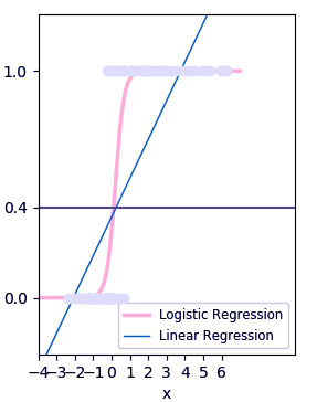
>>> plt.scatter(x.ravel(),y,color=’lavender’,zorder=17)


<matplotlib.collections.PathCollection object at 0x057B0E10>


قطعه کد ۲:

>>> x_test=np.linspace(-7,7,277)
>>> def model(x):
return 1/(1+np.exp(-x))
>>> loss=model(x_test*clf.coef_+clf.intercept_).ravel()
>>> plt.plot(x_test,loss,color=’pink’,linewidth=2.5)


[<matplotlib.lines.Line2D object at 0x057BA090>]


قطعه کد ۳:

>>> ols=linear_model.LinearRegression()
>>> ols.fit(x,y)


LinearRegression(copy_X=True, fit_intercept=True, n_jobs=1, normalize=False)

قطعه کد ۴:

>>> plt.plot(x_test,ols.coef_*x_test+ols.intercept_,linewidth=1)


[<matplotlib.lines.Line2D object at 0x057BA0B0>]


قطعه کد ۵:

>>> plt.axhline(.4,color=’.4′)


<matplotlib.lines.Line2D object at 0x05860E70>

قطعه کد ۶:

>>> plt.ylabel(‘y’)


Text(0,0.5,’y’)

 قطعه کد ۷:
 
>>> plt.xlabel(‘x’)
 
Text(0.5,0,’x’)
 
قطعه کد ۸:
>>> plt.xticks(range(-7,7))
>>> plt.yticks([0,0.4,1])
>>> plt.ylim(-.25,1.25)
 

(-۰٫۲۵, ۱٫۲۵)

قطعه کد ۹:

>>> plt.xlim(-4,10)


(-۴, ۱۰)

قطعه کد ۱۰:

>>> plt.legend((‘Logistic Regression’,’Linear Regression’),loc=’lower right’,fontsize=’small’)


<matplotlib.legend.Legend object at 0x057C89F0>


قطعه کد ۱۱:

>>> plt.show()

رگرسیون لجستیک

اگر نوشته بالا برای شما مفید بوده است، آموزش‌های زیر نیز به شما پیشنهاد می‌شوند:


منبع [+]

پاسخی بگذارید

نشانی ایمیل شما منتشر نخواهد شد. بخش‌های موردنیاز علامت‌گذاری شده‌اند *